模拟退火算法(Simulate Anneal,SA)是一种通用概率演算法,用来在一个大的搜寻空间内找寻命题的最优解
模拟退火算法原理
模拟退火(Simulated Annealing简称SA)算法是基于蒙特卡罗迭代算法求解的一种启发式随机搜索算法,算法思想最早在1953年由N·Metropolis等人提出的。算法出发点是物理学中的退火过程,即对固体物质进行退火处理时,通常足先将它加温,使其粒了可自由运动,然后降温,粒子逐渐形成低能态的品体,若在凝结点附近温度下得足够慢,则固体物质一定会形成域低能量的基态。
模拟退火算法的基本思想是从一个给定解开始,从邻域中随机产生另一个解,接受Metropolis准则允许目标函数在有限范围内变坏,它由控制参数t决定,其作用类似于物理过程中的温度T,对于控制参数的每一取值,算法持续进行“产生-判断-接受或舍去”的迭代过程,对应着固体在某一恒定温度下的趋于热平衡的过程,当控制参数逐渐减小并趋于0时,系统越来越趋于平衡态,最后系统状态对应于优化问题的全局最优解。
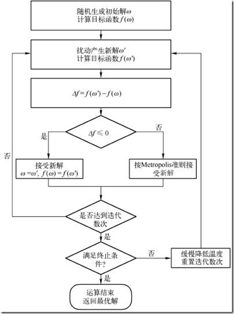
模拟退火算法流程
(1) 给定模型每一个参数变化范围, 在这个范围内随机选择一个初始模型m0, 并计算相应的目标函数值 E(m0) 。
(2) 对当前模型进行扰动产生一个新模型 m, 计算相应的目标函数值E(m), 得到 ∆ E = E(m)-E(m0).
(3) 若 ∆E<0, 则新模型被接受; 若∆E>0, 则新模型 m 按概率P= exp(∆ E/T)进行接受,T为温度。当模型被接受时, 置m0=m,E(m0)=E(m)。
(4) 在温度T下, 重复一定次数的扰动和接受过程, 即重复步骤(2)、(3)。
(5) 缓慢降低温度 T 。
(6) 重复步骤(2)、(5), 直至收敛条件满足为止。
非线性规划方程求解
题目
1 |
|
MATLAB代码
1 | clear |
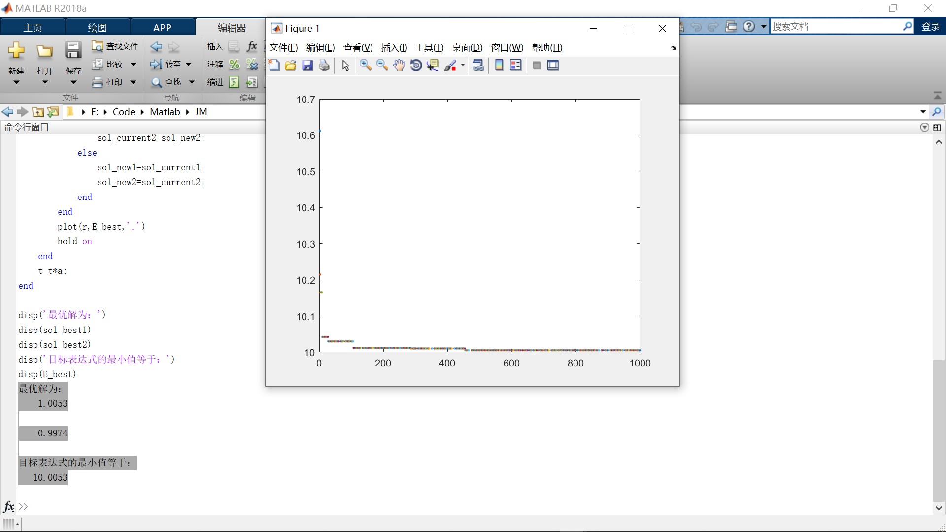
运行结果
1 | 最优解为: |